Thoughts on deep learning training.

Improving Single Device Training Performance

Techniques for memory considerations

• Mixed Precision Training

  Mixed precision training speeds up training by using 16 bit weights while maintaining a 32 bit copy of weights for high precision inference. During training, weights are rounded off to 16 bit representations and gradients scaled up to make them significant in 16 bit precision. During the update step on the 32 bit master copy of the weights, the gradients are scaled down to restore their original value. Using 16 bit weights for training leads to a lower memory requirement for storing activations.

• Gradient Checkpointing

  Instead of storing all intermediate activations (to be used during the backward pass), one mays store only some of the intermediate activations (checkpoints) and recompute the others (by doing a forward pass from the checkpointed activations) everytime they are needed.

  Gradient checkpointing can be a trade-off that reduces memory consumption but increases compute requirement.

Techniques for training time considerations

• Second-order Optimization

  First-order optimization methods take time to converge, as first derivates often do not capture the loss surface very well. Second-order optimization methods are more accurate but they require costly matrix inversion operations. Techniques like Kronecker Factored Approximate Curvature K-FAC enable inexpensive second-order optimization as the creatively factorize out large matrices into smaller block matrices. For more details visit here

• BatchNorm:

  Batch norm reduces the effects of second-order interactions between weights in different layers, thus stabilising gradient values and speeding up convergence.

  Note : A common misconception is that the use of BatchNorm makes usage of L2 regulariation redundant as the activations are renormalized anyway. It is important to note that while BatchNorm normalizes activations the weight are free to grow in magnitude. Hence, L2 is still important to keep the weights bounded within a fixed radius hypersphere.

• Prioritized Sample Batching:

  Reinforcement learning techniques like DDPG use a concept called Prioritized Experience Replay to select samples with highest prediction error to train the policy network. The same fundamental concept could be used in general supervised learning to select those samples (to be a part of the next batch) that have the highest loss, and can provide the most useful gradient update.

  A way to do that would be a Metropolitan Hastings style method (discussed here) wherein the next samples for a batch are chosen based on a Markov chain starting from the current batch’s samples. The probability distribution over the next set of samples in the Markov chain could be defined as a ratio of the losses. Once the samples are chosen their losses could be weighted via importance sampling weights so that they do not overcorrect the network.

Improving Multi Device Training Performance

• Data vs Model Parallelism

  Data Parallelism is preferred when we have lots of data that can’t fit on a single device and exchanging weight gradients is relatively easier (especially in case convolutions where kernels have relatively few parameters).

  On the other hand, Model Parallelism is preferred when there are too many parameters to be fit on a single device and exchanging activation gradients is easier.

• Asynchronous Optimization

  Asynchronous gradient descent with multiple workers is the bedrock of techniques like A3C in reinforcement learning. The parameters to be updated are stored in shared memory and updated by each worker asynchronously. Since each worker has access only to a subset of the whole training data, the gradients are not very accurate and are noisy. However, gradients in deep learning are anyways noisy and this technique provides a decent speedup.

• Reduce

  Anytime distributed training happens, there is a need to accumulate all gradients from all GPUs via a reduce operation. For large models, this can be a bottleneck step if gradients are accumulated sequentially from each GPU or if they cause latency issues due to lower inter-GPU memory bandwidth. There are a number of creative reduce techniques that avoid the issues. Two famous ones are mentioned below.

  Baidu’s RingReduce descriptively written about by Andrew Gibiansky. You can find my PyTorch-based implementation of Baidu’s RingReduce here.

  Reduction Tree as described in the FireCaffe paper by Iandola et. al.. It is essentially a binary tree performing reduce operations in parallel (each process handles two GPU nodes at a time ) with O (log N) complexity.

Other Techniques

Finding good hyperparameters is essential for pain-free training routines. A relatively new method developed by DeepMind is Population Based Training (PBT).

• Population-Based Training

  Population-based training is essentially employing evolutionary algorithms to hyperparameter search wherein an ensemble of models is trained with each having their own set of hyperparameters that keeps evolving, transferring after certain intervals through the training procedure. It does seem to be the most efficient AutoML/Neural Architecture Search method so far. More recently it has been used by Waymo in training their NN models and searching for good data-augmentation policies to train their vision pipeline.

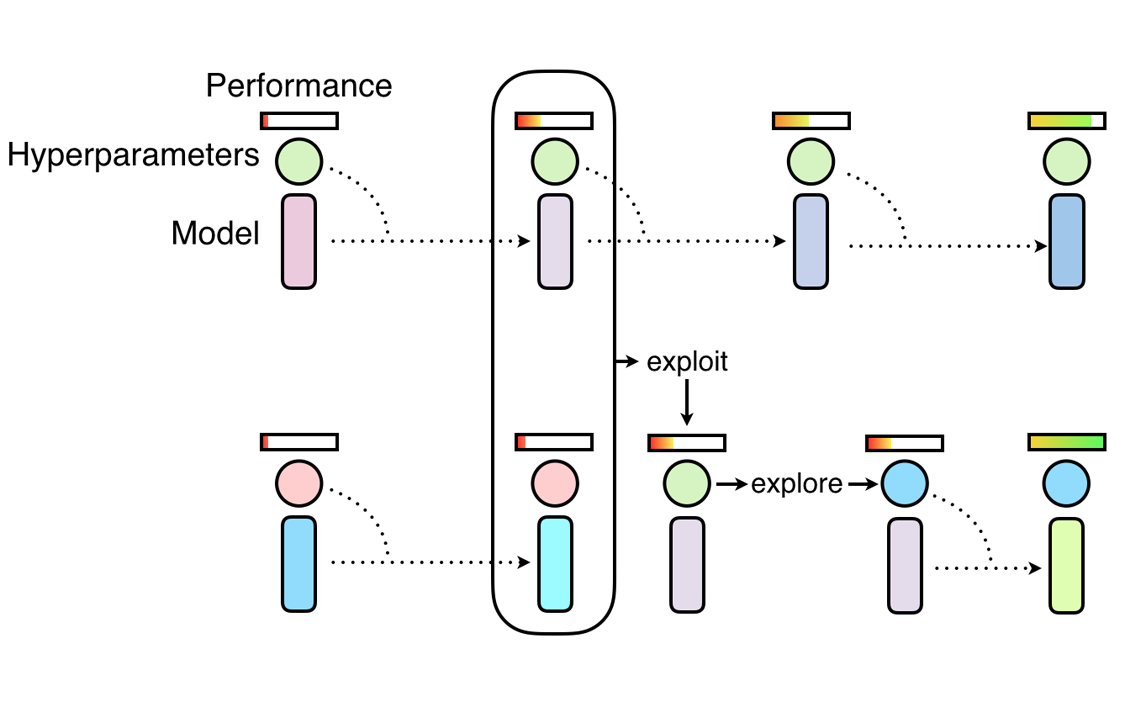  An overview of how top performing models keep mutating and the bottom performs adopt the top performers’ parameters.Credits: DeepMind

  A crude pseudocode to implement it is provided below.

def hparam_search(models, K, perturbation):
    N = len(models)
    while max(scores) < MAX_SCORE:
        start training N different models
        ranked_models = sorted(models, lambda model: score(model))
        top_models = ranked_models[:K]
        bottom_models = ranked_models[K:]
        
        for model in bottom_models:
            top_model = random.choice(top_models)
            model['state_dict'] = top_model['state_dict']
            model['optimizer_state'] = top_model['optimizer_state']

        for hparam in hparams:
            for model in top_models:
                model[hparam] += perturbation